Week 4: Data cleaning and processing with R/RStudio
The goal of this session is to start to learn about data wrangling – we saw last week how to gather data and today we will see how to transform it. This is key to being able to then analyse and explore the data and in practice the data wrangling part is probably about 80% of the effort when dealing with real life datasets.
Learning objectives
- To show you how to manipulate data using the dplyr package
- To show you how we can join two datasets (or tables) using a common variable
- To highlight potential issues when working with real datasets (e.g. outliers andmissing values)
1. Recap
Over the past three weeks we have learned some of the basics of R including how to run functions, working with various types of data structure (e.g. vectors and data frames) and last week reading datasets and do some visualisation. This week we will focus on working with data and in particular transforming data. We also looked at the concept of packages in R which extend the base functionality. We will utilise another tidyverse package especially designed for data wrangling called dplyr. This all forms a part of the data exploration process.
2. Data transformation with dplyr packages
Okay so we know how to load data into R and RStudio, but one of the most important aspects of ‘data wrangling’ is data transformation; that is filtering and selecting data; ordering data etc. We did some of this in Week 2 when we looked at data frames (the main data structure used in R when doing data science). However, if we remember this it was quite hard going and tidyverse provides the dplyr package that is a far easier set of tools for data transformation. RStudio provides ‘cheat sheets’ for commonly used packages and this includes dplyr:
https://www.rstudio.com/wp-content%2Fuploads%2F2015%2F02%2Fdata-wrangling-cheatsheet.pdf
These are the main dplyr functions for working on data frames:
- Pick observations by their values -
filter() - Reorder the rows -
arrange() - Pick variables by their names -
select() - Create new variables with functions of existing variables -
mutate() - Collapse many values down to a single summary -
summarise()
We will use the mpg dataset (you might remember it from practicals of INF4000) that comes in-built with tidyverse. The dataset contains information about cars and consists of the following columns:
To read more about this dataset: https://rdrr.io/cran/gamair/man/mpg.html.
It is also worth highlighting at this stage a very useful dplyr function which is called ‘piping’ where we can pass the output of a function as the input to a next command using %>%. This saves a lot of time as you don’t need to keep storing results in variables. We’ll see the use of this in a moment.
Selecting rows/observations - filter()
Suppose we want to select the rows (or observations) from the mpg dataset where the manufacturer is Audi. We can use the filter() function for this:
We could instead filter data where the engine displacement (displ) is greater than 2 (i.e. >2):
Similarly we could select vehicles with engine displacement (displ) is greater than or equal to 2 (>=2):
We can create more complex matching conditions using logical operators (see Week 2). For example, selecting the rows where the engine displacement is greater than 2 and (use &) the number of cylinders is greater than 6:
You could select Audi cars built in 1999 using either of these function calls to filter():
Note that in the first command we see the variables separated by ‘,’ and in the second we use ‘&’ - they both produce the same results.
Exercise
can you filter rows where the manufacturer is Audi OR the year of production (year) is 1999? Can you filter rows where the year of production (year) is 1999 and the manufacturer is NOT Audi?
Suppose we now want Audi or Chevrolet cars from 1999; we can create this using the following command:
If you look at the RStudio cheatsheet you can see the entire range of logic functions you can use (see “Logic in R” at the bottom of the sheet). One that is useful is the %in% logic comparison for group membership. We could have carried out the above also using %in% and a vector of names:
To show the use of the dplyr pipe command (%>%) we could pass the output of the previous filter() function as the input to the count() function where we want to count the manufacturer, i.e. how many Audi and Chevrolet cars were released in 1999:
On the RStudio cheatsheet you can find some other very helpful subset functions to filter out rows from a data frame (or tibble). This includes the common task of selecting a random sample of observations or rows. For this we can use the sample_frac() function (to sample a proportion of the rows) or sample_n() function (to sample a number of rows):
The replace=TRUE in the functions means that when a row is selected (taken out of the dataset), it is replaced by a copy. What this means, is that it is possible that the same row is chosen more than once. If you don’t want this, don’t write it, the default is not to replace. Notice that every time you run the function, it will provide different results. If you want to make results consistent, you can use the function set.seed(X), where X is a number, before calling the sample function.
Reordering rows - arrange()
We’ll make use of the 2016 Rio Olympic Games medals table to show how we re-order rows using the arrange() dplyr function:
We can order by multiple columns simply adding more columns to the arrange() function as parameters. It can be hard to see this in action so we’ll order the data by number of gold, silver and bronze medals, but we will need to inspect the ties (i.e. where the values are the same) to be able to see the ordering by different columns. Let’s arrange the rows by number of gold medals won, followed by silver and then bronze (in descending order):
You can see the ordering with multiple columns where the preference is Gold but when we have the same number of gold medals (e.g. from row 9 and 10) then the data is sorted by number of Silver medals.
Exercise
to better view the ordered tibble, pipe the results of the arrange function into the function View. Make sure that ties between countries with the same number of gold and silver medals are sorted based on the number of bronze medals.
Selecting columns - select()
Selecting columns with dplyr is very simple using the select() function. To select from the mpg dataset the manufacturer and highway fuel efficiency (hwy) columns we use:
It you look at the RStudio cheatsheet you will see (bottom right) a series of ‘helper’ functions. These can be used with the subset() function and used for selecting columns. For example, we could select all the columns that begin with ‘d’:
What’s useful is that using the pipe %>% command we can then use the commands select() and filter() together to filter out rows and columns
Note if we wanted to find all manufacturers other than Chevrolet where hwy >= 20 we could use the logical NOT ! operator:
We could keep combining commands using the pipe %>% command to also arrange the data, e.g. in descending order of manufacturer:
Finally, note how each the functions we have seen can work without specifying the data if they are part of a pipe chain. That means you can also start with your data and then chain all the functions. For example, the command below works the same as the previous one:
Creating new variables - mutate()
The mutate() function allows making new variables that are typically based on existing variables. For example, in the Rio 2016 medals data we could create a new column/variable for the total of medals won using the mutate() function:
Note that the mutate function doesn’t change the original data, which means the new column is only available to functions that are piped after the mutate. If you want to save the new column, you will need to save the result of mutate to a variable. Also note that if you create a column with the same name as an already existing one, it will overwrite the existing one.
Collapse many values down to a single summary - summarise()
The summarise() function allows us to summarise data into a single row of values. For example, we could compute the average of highway efficiency (hwy) of the mpg dataset using the following summarise() command:
Notice that like mutate, summarise creates a new column. Often the summarise() function is paired with the group_by() function. So let’s suppose we want to group the mpg data by manufacturer and year then we can do this with the following group_by() function:
We could use the group_by() and summarise() functions together (with a pipe) to count the number of rows we have for each manufacturer using the n() function (which stands for number):
Exercise
Look at the second page of cheatsheet for useful functions to use with mutate and summarise. How many unique models do each manufacturer produce? Create a new column with a ratio of highway efficiency (hwy) vs city efficiency (cty) called HwyCtyRatio.
3. Combining datasets
There are many ways of combining datasets, which is a common task in data science and you may have to do that in your coursework. Multiple functions are available for this and we will come back to this later in the course but dplyr makes use of the notion of joins from relational databases to combine datasets.
There is an excellent overview of this in Chapter 10 of R for Data Science (which is Chapter 13 in the online version: http://r4ds.had.co.nz/relational-data.html). We will come back to joining datasets later in the course because we need to spend more time on this, but for now let’s get a quick flavour of what we can do in R with dplyr.
Note: don’t worry if you don’t understand all of this yet as you will also learn about relational data next semester in the Database Design module.
To demonstrate joining datasets let’s make use of a package called nycflights13 which contains various tables of data which are what we call relational - the tables are related to each other in some way (via keys):
Note that the use of :: is the R way of identifying functions (or datasets) within a package. We can also view other datasets:
The airlines data frame is a table of airline numbers and names; the flights data frame contains flight details. To make things easier let’s drop unimportant variables so it’s easier to understand the join results - we can use a select() function for this:
Suppose we want to have the full name of the airline in the flights2 table rather than the carrier abbreviation. We have the abbreviation and the full name in the airlines table and therefore we can combine tables using a join command.
In the airlines table you have the full name of the airline carrier listed once - abbreviation and number (e.g. AA is American Airlines Inc.). What we want to do is to go through each of the rows in the flights2 table and match the carrier abbreviation with the carrier in the airlines table replacing the abbreviation with the name as we go.
The left_join() function is an example of a mutating join: “A mutating join allows you to combine variables from two tables. It first matches observations by their keys, then copies across variables from one table to the other” (Wickham & Grolemund, 2017: 181). The idea of a join between tables is that you combine data using a key variable - in this case by the carrier abbreviation. That key variable needs to be present in both tables, ideally using the same column name. There are different types of join including inner and outer joins. We have used an outer join which means that any rows appearing in at least one of the tables being joined is kept. Figure 1 shows three types of outer join: left, right and full with the keys for joining being 1, 2, 3, etc. In outer joins, at least one of the tables (or both in full outer join) keep all of its records. When a row contains a value for the key variable that is not present in the other table, the new column is filled with missing values. Inner joins only match records that are present in both tables and is the most frequent joined you will use in the Database Design module.
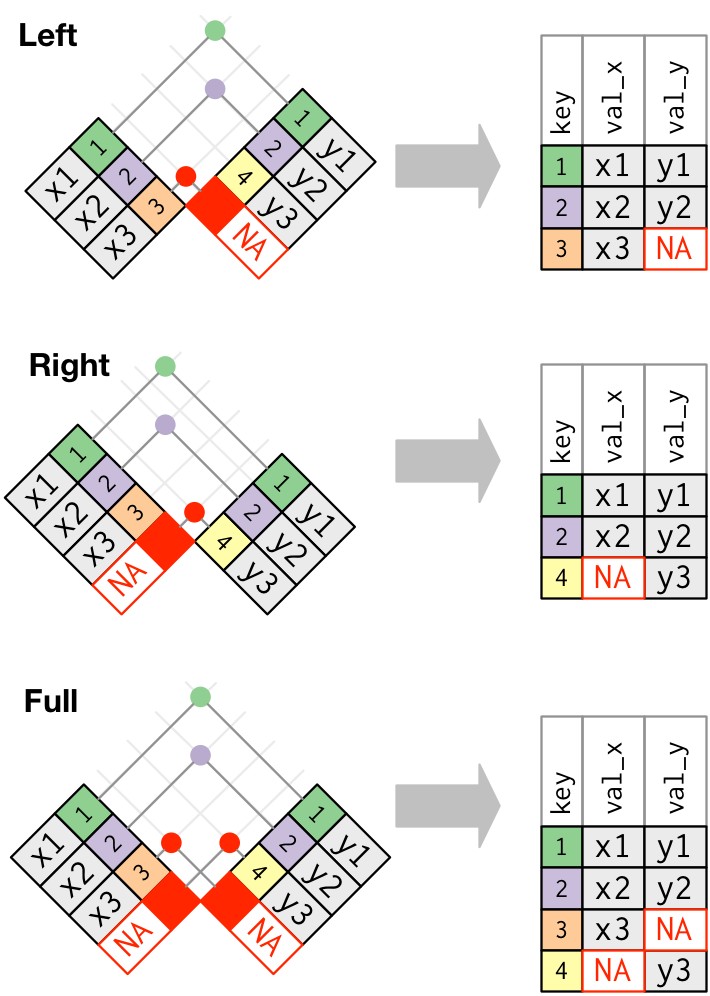
In our case we used a left join which means we keep all the observations in the flights2 table (i.e. we don’t ‘lose’ any of the flights) and where carrier matches in the airlines table the carrier name is copied across as a new variable (or column) in the flights2 table.
Again, we will come back to combining datasets in a later session so don’t worry too much about this for now, but do be impressed by what you can do with dplyr because it’s very powerful.
4. Working with real data
Finally, let’s just return to the Free School Meals (FSMs) dataset that we worked on the previous week (you can find the file on the week 3 practical folder). Much of the data we have worked with so far is what we might call clean - it’s fairly complete and in a useable format. But the FSM dataset is more realistic of what we might find in practice. There are at least a couple of ‘features’ to point out with this dataset. Start by viewing the dataset:
If you scroll through the data a couple of things might stand out to you:
- There seems to be a repeated high value (9999) in the FSMTaken column
- There is a value of NA also in the FSMTaken column
Viewing the data.go.uk page about the dataset (https://data.gov.uk/dataset/free-school-meals) we see an explanation for this:
Please note that, due to data protection requirements, we can’t publish real values
for FSMTotal or FSMTaken when those figures are < 5. Thus, those values have been converted to 9999. If a cell has no value it means that data is not collected for that field for that specific school.
It’s important to know your data and in this case identifying that 9999 is a ‘fake’ value is important, especially if we compute functions (e.g. averages) across the values; if we treat 9999 as an actual value we will get inaccurate results. The other issue is with the NA (Not Available) values - these represent missing data and this is something that comes up a lot in practice. To see the effects of these let’s assume we want to compute the mean number of FSMs taken across all schools in our dataset. Start with getting a summary of the values using the summary() function:
We see that the mean is very different from the median and the maximum value of FSMTaken is 9999. The big difference in the mean and median signals a potential problem and the mean value is being affected by outliers (i.e. the 9999 value). The summary() function also tells us we have 17 missing values (NA).
We can also experience problems if we try to use the mean() function on the FSMTaken column:
The problem here is that we have missing values and the mean() function by default doesn’t like this. We can ignore the missing values using the na.rm=TRUE parameter in the mean() function (i.e. this says remove any NA values when computing the mean):
But again the mean seems very high and we know that this is not a true value because of the 9999 value. Therefore we should ignore these rows when computing the mean. You might need to go back to Week 1 where we looked at vectors , but we can filter out values using this command:
The original FSMTaken column contained 250 values; we’ve removed the 9999 values and now we can compute the mean:
This is an accurate mean value and you can confirm this because it is far closer to the median value.
In R there is always more than one way to do something. Now you might have said why not use the dplyr function select() to filter out rows where FSMTaken is 9999. We could do this using:
If we then count the number of rows in the filtered dataset we see we have 189 rows:
Why doesn’t this match the 206 value when we counted the number of values in actualFSMTaken? It’s because the filter() command has also removed the data with the NA values (206-17=189). We could keep the NA values using filter() in this way:
The above says filter and return values of FSMTaken that are less than 9999 OR where the value is NA - this is achieved using the is.na() function which returns TRUE if the value is NA.
The final question for the moment is what do we do with missing values? One approach is to simply ignore rows (or columns) where we have missing values. But this means we could be throwing away a lot of our data. There are various ways of handling missing data, including replacing NA with a mean value, learning a model/function to estimate a value, insert a random value, etc. For more information see:
- https://thomasleeper.com/Rcourse/Tutorials/NAhandling.html
- http://www.dummies.com/programming/r/how-to-deal-with-missing-data-values-in-r/
One approach could be to replace the NA value with a mean value. As a simple example suppose we create a vector of 4 elements with the last value being NA:
Remember in R that many functions are vectorised - this means that they are executed on each element of a vector. So in the above R will go through each element and test if the value is NA and if it is then replace this element with the mean value of y. So the mean of 4, 5 and 6 if 5 which is used to replace the element with the NA value (element 4). Let’s do this on our actualFSMTaken vector:
You can check this works for yourself (e.g. check the 4th value from the last element in the vector). The floor function is useful to transform the mean value from a double (29.90476) to an integer (29) so there is no mismatch with the over values.
This is okay but what if we want to work with the original data frame and keep all the values (rather than extract out a vector of just the FSMTaken column)? We can use the dplyr mutate() function to create a new variable called newFSMTaken in our existing data frame. For now let me show you how to do this as it may appear confusing at first:
I have omitted some rows above but if you check row 40 you can see that the NA has now been replaced with the mean value 29.
You haven’t seen the ifelse() statement1 before. This is called a condition and is very helpful as it controls when we do things. This basically says if condition==TRUE (the value of FSMTaken is NA) then assign value A (the mean of FSMTaken as an integer); else assign value B (the value that is already present because it is not NA). In our example: if the FSMTaken value is NA then we compute the mean of FSMTaken and use this value; otherwise we use the original FSMTaken value. Using mutate() we assign this to a new variable called newFSMTaken.
Exercise
Lets imagine someone asks you to obtain the mean of FSMTaken in the worst case scenario, where all the 9999 values (when the value is less than 5) are considered to be 4. Use the functions you have learned today to change those 9999 values to 4 (probably best to create a new column for this) and calculate the mean. Do the same thing, for the case scenario where FSMTaken for those 9999 values is considered to be 0.
Further resources
Specifically for this session:
- R for Data Science - from the book (Chapters 3, 8 and 10)
- R for Data Science - from the website (Chapters 5, 11 and 13)
- Learning R book (Chapters 12 and 13)
- The RStudio cheatsheet for data wrangling: https://www.rstudio.com/wp-content/uploads/2015/02/data-wrangling-cheatsheet.pdf
- Datacamp tutorial on importing data: https://www.datacamp.com/community/tutorials/r-data-import-tutorial
- See the links throughout this handout
For more information about working with Excel files see: https://www.datacamp.com/community/tutorials/r-tutorial-read-excel-into-r There are packages and functions for reading data into R for most formats, see e.g.: http://www.statmethods.net/input/importingdata.html and https://www.datacamp.com/community/tutorials/r-data-import-tutorial
More generally:
- Swirl interactive tutorial on R: https://github.com/swirldev/swirl_courses
- R for Data Science: http://r4ds.had.co.nz/